
- Select the Currency button in the Number section of the Home tab. Choose More Accounting Formats. With Custom highlighted as a category, select the Symbol drop-down on the right. Select Japanese from the list currency symbols that appear.
- Select the Currency button in the Number section of the Home tab. Choose More Accounting Formats. With Currency highlighted as a category, select the Symbol drop-down on the right. Select Japanese from the list of currencies that appear.
- Select the Currency button in the Number section of the Home tab. Choose More Accounting Formats. With Special highlighted as a category, select the Symbol drop-down on the right. Select Japanese from the list of currency symbols that appear.

- On the Format choice in the Editing group.
- On the Format choice in the Styles group.
- On the Format choice in the Cells group.

- The number format is incorrect.
- The cell contains text and numbers.
- The column is too narrow.

- The Comma format
- The Percentage format
- The Currency format

- Select column G and click Format on the Home tab. Choose Hide & Unhide from the drop-down menu and then unhide columns from the sub-menu.
- Select the column to the right of the hidden column. Select Format on the Home tab. Choose Hide & Unhide from the drop-down menu and then unhide columns from the sub-menu.
- Highlight columns F and H. Select Format on the Home tab. Choose Hide & Unhide from the drop-down menu and then unhide columns from the sub-menu.

- Type the word Name in the cell underneath the heading.
- Use the Center align command in the Alignment group on the Home tab.
- Use the Wrap Text command in the Alignment group.

- The Contextual Sort tab
- The View tab
- The Data tab
- Select Product Name from a drop-down list.
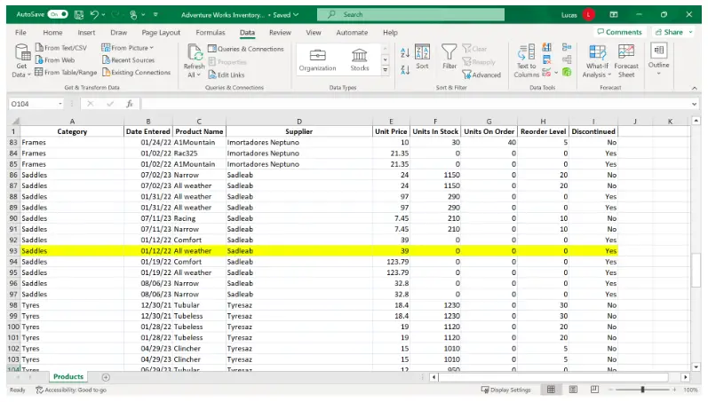
- Select any cell in column C.
- Select column C by selecting the column initial.
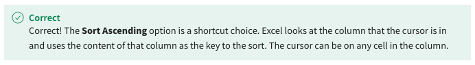
- Sort
- Sort A to Z
- Sort Z to A

- True
- False
- Use the Clear option on the Data ribbon.
- Use the Undo button.
- Use the Clear filter from choice in each filter drop-down.
- Check the bottom-right of the Excel Screen.
- Check the bottom-left of the Excel screen.
- Check the middle of the status bar.
- You selected Text filter and then begins on the sub-menu.
- You selected Text filter and then equals on the sub-menu.
- You selected Text filter and then contains on the sub-menu.

- The Name Box
- The Title Bar
- The Formula Bar

- The Filter arrow drop-down symbol is in bold.
- The Filter arrow contains an arrow symbol.
- The Filter arrow contains a funnel symbol.

- At the top of the column.
- At the bottom of the column.
- In the middle of the column.
- Freeze Panes
- Freeze Top Row
- Freeze First Column

- True
- False
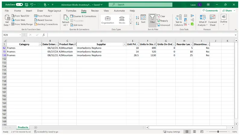
- Use Begins with on the Text Filter sub-menu.
- Use Ends with on the Text Filter sub-menu.
- Use Contains on the Text Filter sub-menu.
- Tick the box that says, My data has headers.
- Select the whole data range.
- Click the first row of the data range.

- MonthlyProfit2

- Monthly Profit
- Monthly_Profit
- The Review ribbon.
- The View ribbon.
- The Home ribbon.

- The calculation.
- The result.
- The calculation and the result.
- There is a darker vertical line between two of the column initials.
- There is a gap in the initial letters at the top of the screen.
- Some column initials are shaded in a different background color.

- An arrow.
- A white cross.
- A narrow black cross.

- Format drop-down.
- Insert drop-down.
- Delete drop-down.
- True
- False
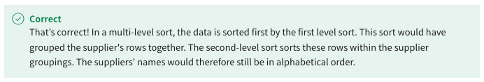
- Select Add and choose Product from the then by order column.
- Select Add and choose product from the then by column drop-down.
- Select Add and choose Supplier from the Then by column drop-down.
- Select the Insert Ribbon, select on Insert, and then select Insert Sheet Columns.
- Click the right mouse button, select Insert, and then select Entire column.
- Select the Home ribbon, select Insert, and then select Insert Sheet Columns.
- In the Alignment group on the Home ribbon.
- In the Editing group on the Home ribbon.
- In the Number group on the Home ribbon.
- Use the Clear option in the Filter group in the Data Ribbon.
- Use the Clear Filter option on the Filter menu in the Name column.
- Use the Clear Filter option on the Filter menu in the Town column.

- Use Begins with on the Text Filter sub-menu.
- Use Equals on the Text Filter sub-menu.
- Use Ends with on the Text Filter sub-menu.
- Use the Name box on the top left of the worksheet.
- Use the Search feature at the top of the Excel window and type the name.
- Use the Name Manager in the Formulas ribbon
- Point at the sheet tab. Hold down the Ctrl key and then the mouse button. Drag the sheet to a new location.
- Point at the sheet tab. Hold down the mouse button. Drag the sheet to a new location.
- Point at the sheet tab. Click the right mouse button. Choose Move or Copy from the shortcut menu.
- The content will only be partially displayed and some of the entry will be hidden by the content in B2.
- The content will be replaced by crosshatch symbols as the column is too narrow to display it fully.
- The content will automatically “wrap around” so that some of the heading will be brought down to a new line.